Chapter 7 - Machine Learning Foundations (First Time Learners, Weeks 7-12)#
Try it | Goals: fully and solidly learn four things - how an image becomes numbers (features) -> how a model learns to judge -> how to prevent cheating -> how to tell if a model is good. We start from a point of view that someone who has never touched machine learning can follow, with real-data figures, progressing step by step without rushing.
7.0 Chapter Roadmap: How to Study (about 3-6 weeks)#
If you have a 6-12 month cycle, treat this chapter as a real first course in machine learning, not a crash course to “understand the project code.” Suggested path:
Step 1 (~1 week): read only 7.1-7.2, build the “data -> features -> labels” picture, and be able to name everyday examples of “describing an image with numbers”.
Step 2 (~1 week): read 7.3-7.5 with Fig. 7-1/7-2/7-3, understand “draw a line + turn the line into probability + make the probability right”. No formula derivation required, just be able to retell the idea by looking at the figures.
Step 3 (~1 week): read 7.6-7.8, focus on data leakage and how to evaluate. This is where real projects most often stumble, and it deserves extra time.
Step 4 (~1 week): run every code excerpt on your own machine (
python src\train_model.py) and confirm where each output number comes from.
How to study | Every section ends with a “Think about it”. Write the answer down rather than just thinking in your head - writing is where real learning happens.
7.1 Steganalysis Is Just “Is This Image Hiding Something?”#
Change perspective: a photo is either clean (marked 0) or had a message hidden in it (marked 1). Machine learning just learns a judgment: give it an image and try to guess 0 or 1.
This is like a teacher giving students many problems with answers, and then students solve unseen problems on a test - machine learning does not “memorize”, it learns the rule. Supervised learning has four pieces: data, features, model, evaluation. We go through each, mapping every one to project code.
Mini-glossary | You will see these four words throughout. First remember their “plain” version:
Data: a pile of “examples with answers”.
Feature: the short list of numbers an image is compressed into (like “measuring the image with rulers”).
Model: a “features-to-answer” judgment rule.
Evaluation: judging whether that rule is reliable.
7.2 How an Image Becomes Numbers: Features and Labels#
A computer does not “see” images, only numbers. So step one is to compress an image into a short list of numbers. The project’s v1 compresses each image into 11 numbers, and v1.4 extends this to 143 (Chapter 8). Those 11 numbers are the feature vector - like “measuring the image with 11 rulers.”
Feature: the 11 numbers (e.g., “how chaotic the pixel differences are”, “is the brightness distribution off”).
Label: whether the image hid something; 0 = clean, 1 = hidden.
Sample: one row = one image, 11 feature numbers + 1 label.
What the dataset looks like (first columns are features, label is the answer, ignore photo_id for now)
Rm,Sm,Rn,Sn,RS_Gr,RS_Gn,chi2_pvalue,diff_entropy,lsb_diff_entropy,median_prefix_p,chi2_stat,label,photo_id,...
41316,4574,36608,5057,0.56,0.48,0.56,1.99,0.986,2.7e-166,1719.3,0,0,...
40488,4907,35701,5342,0.54,0.46,0.61,2.02,0.989,2.2e-155,1675.9,1,0,...
data/dataset.csv (real first two rows, numbers truncated for display)
Tip | Do not panic at names like
chi2_pvalueorRS_Gn. They are just “the number from ruler number N.” Chapter 8 explains what each ruler measures.
Write the table as notation - every formula below uses it (do not fear; it is just “row i, column j”):
Sample: one row is one sample, \(N\) in total, indexed \(i=1,\dots,N\);
Features: the 11 numbers of sample \(i\) are a vector \(\mathbf{x}_i\); all rows form a matrix \(X\) (\(N\) rows x 11 columns);
Label: \(y_i\in\{0,1\}\), stacked into a vector \(\mathbf{y}\).
7.3 Classification = Draw a Line to Separate Two Groups#
Once we have a pile of “numbers with answers” (features + labels), what does the model learn? It learns to draw a line in number-space: one side clean, one side hiding. Imagine: horizontal axis = “how chaotic”, vertical axis = “is brightness balanced”. Clean images cluster in one corner, hiding images in the other. The model learns that dividing line.
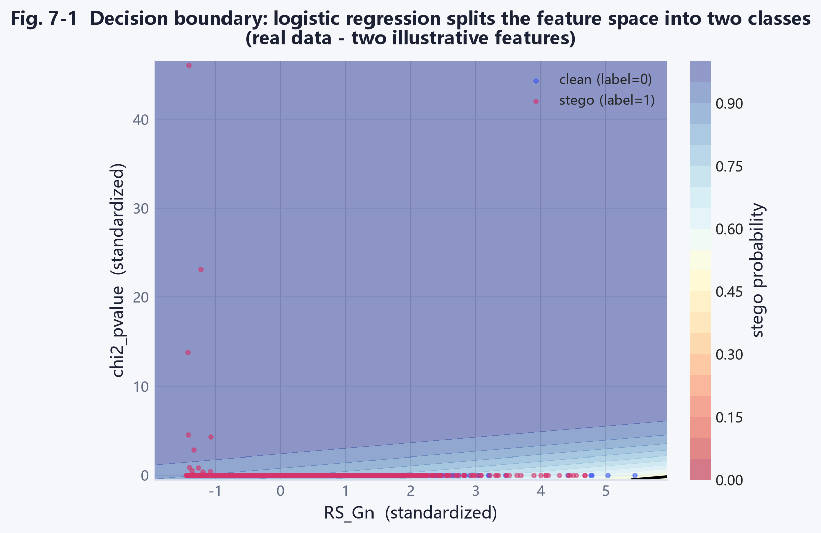
Fig. 7-1 (real data: decision boundary learned by logistic regression on the RS_Gn and chi2_pvalue features; blue = clean, red = hiding, shading = model’s estimated hiding probability)
Understanding this figure is the key to the whole chapter. Notice:
The two classes are not perfectly separable: near the boundary blue and red points mix. The two features are not enough to fully separate, but already “roughly” separate.
The shading is “probability”: the redder, the more the model thinks hiding; the bluer, the more clean. The black line in the middle is the “probability = 0.5” boundary.
More dimensions work the same: the real model uses 11 (or 143) features - it draws a “hyperplane” in 11 (or 143) dimensions. You cannot draw that, but the idea is identical to this 2-D figure.
In math this line is called a linear discriminant function - basically a scoring formula:
Do not let the symbols scare you. It is a weighted sum:
\(x_1,\dots,x_{11}\) are the 11 feature numbers;
\(w_1,\dots,w_{11}\) are weights - they decide “which feature matters and which way the line tilts.” If a feature is especially useful, its \(w\) is big;
\(b\) is the bias - it shifts the whole line up or down to set the position.
Judging is simple: \(z \ge 0\) means “hiding”, \(z < 0\) means “clean”. The single line LogisticRegression is the code that automatically finds the best \(w\) and \(b\).
Think about it | In Fig. 7-1, which of “RS_Gn” and “chi2_pvalue” seems more important for the judgment? If you could keep only one feature, which would you pick? - Your intuition is verified later in the “feature importance” figure in 7.7.
7.4 From Score to Probability: Why a sigmoid?#
\(z\) above is a signed, unbounded “score.” But the user wants a probability between 0 and 1: “how likely is this image hiding something?” So we add a sigmoid that squashes the score to 0-1:
Very large \(z\) (high score) -> \(\hat p\) near 1 (probably hiding);
Very small \(z\) -> \(\hat p\) near 0 (probably clean);
\(z=0\) -> exactly 0.5 (fifty-fifty).
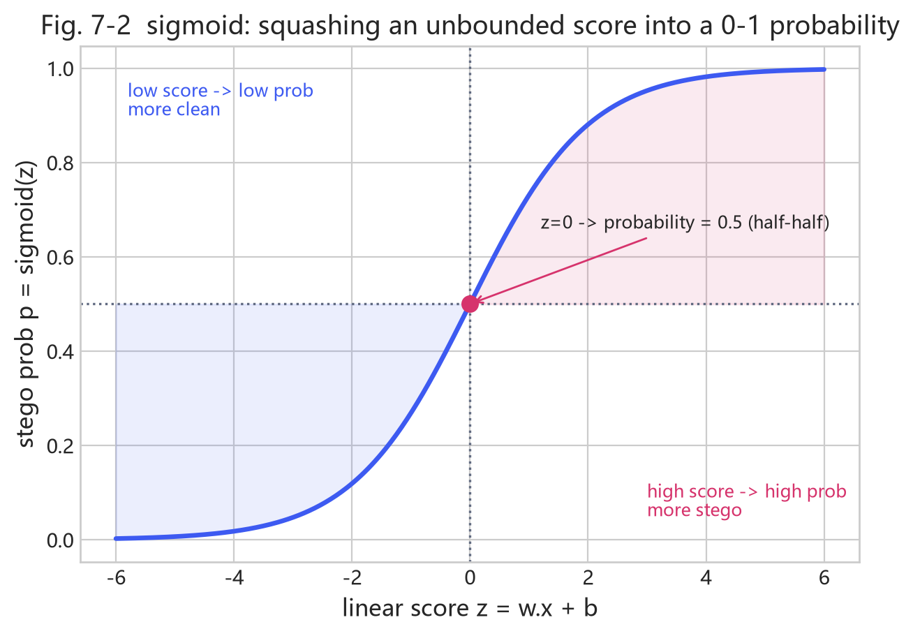
Fig. 7-2 (sigmoid compresses the unbounded, signed “score z” into a 0-1 “probability”. Left blue region = more like clean, right red region = more like hiding)
Tip | Think of sigmoid as a “percentage converter”: it turns a boundary-less score into an easy 0%-100%. Despite the name “logistic regression”, it is still “draw a line + output a probability.”
7.4.1 Why Not Just Output 0/1, but a Probability?#
Good question. Because the real world is not black-and-white. In Fig. 7-1, the points near the boundary are genuinely uncertain. Rather than forcing the model to say “0” or “1”, it is honest to say “I am 73% confident it is hiding.” Then:
The user can choose the threshold themselves (7.7);
You can evaluate how confident the model really is (calibration);
You can draw threshold-independent metrics like ROC / AUC (7.7.1).
Mini-glossary | A classifier that outputs probabilities is soft classification; one that directly outputs 0/1 is hard classification. Logistic regression is soft - that is why it can compute AUC (area under the ROC curve, a measure of how well the model ranks hiding above clean; the higher the better; see 7.7.1).
Against the project code - src/train_model.py.
def lr(seed=0): return make_pipeline(StandardScaler(), LogisticRegression(max_iter=2000, C=0.1, random_state=seed))
Code |
Plain explanation |
|---|---|
|
First make every feature “about the same size”, so a huge number does not skew the line (see 7.4.2) |
|
The “draw a line + sigmoid output probability” above; finds \(w\), \(b\) automatically |
|
Adjust at most 2000 times, so it does not stop early |
|
A dial that says “do not memorise the answers too hard” (regularization, 7.5.2) |
If you want to go deeper | Why standardize? Because the chi-square statistic might be in the thousands while Gn is only 0-1. If the weights treat both equally, the gradient spends all its effort pleasing the big number and the line gets skewed. Standardization is
x'=(x-μ)/σ, turning every feature into “mean 0, standard deviation 1”, so everyone is fair. Note: μ, σ must be computed on the training set only; never sneak the test set in.
7.5 How a Model “Learns”: Loss and Training#
What does “learning” actually do? It keeps adjusting \(w\) and \(b\) so the output probability gets closer to the correct answer. How to measure “close”? Use a loss - think of it as “points deducted for being wrong.” The classic is cross-entropy (log loss):
In plain words: when the true answer is 1 (hidden), only \(\hat p_i\) matters - the closer to 1, the fewer points lost; when the true answer is 0, only \(1-\hat p_i\) matters - the closer to 0, the fewer points lost. The more wrong, the more you lose.
So how to lose fewer points? Try a little bit at a time: compute “which tiny adjustment lowers the loss fastest” and step that way. That is gradient descent:
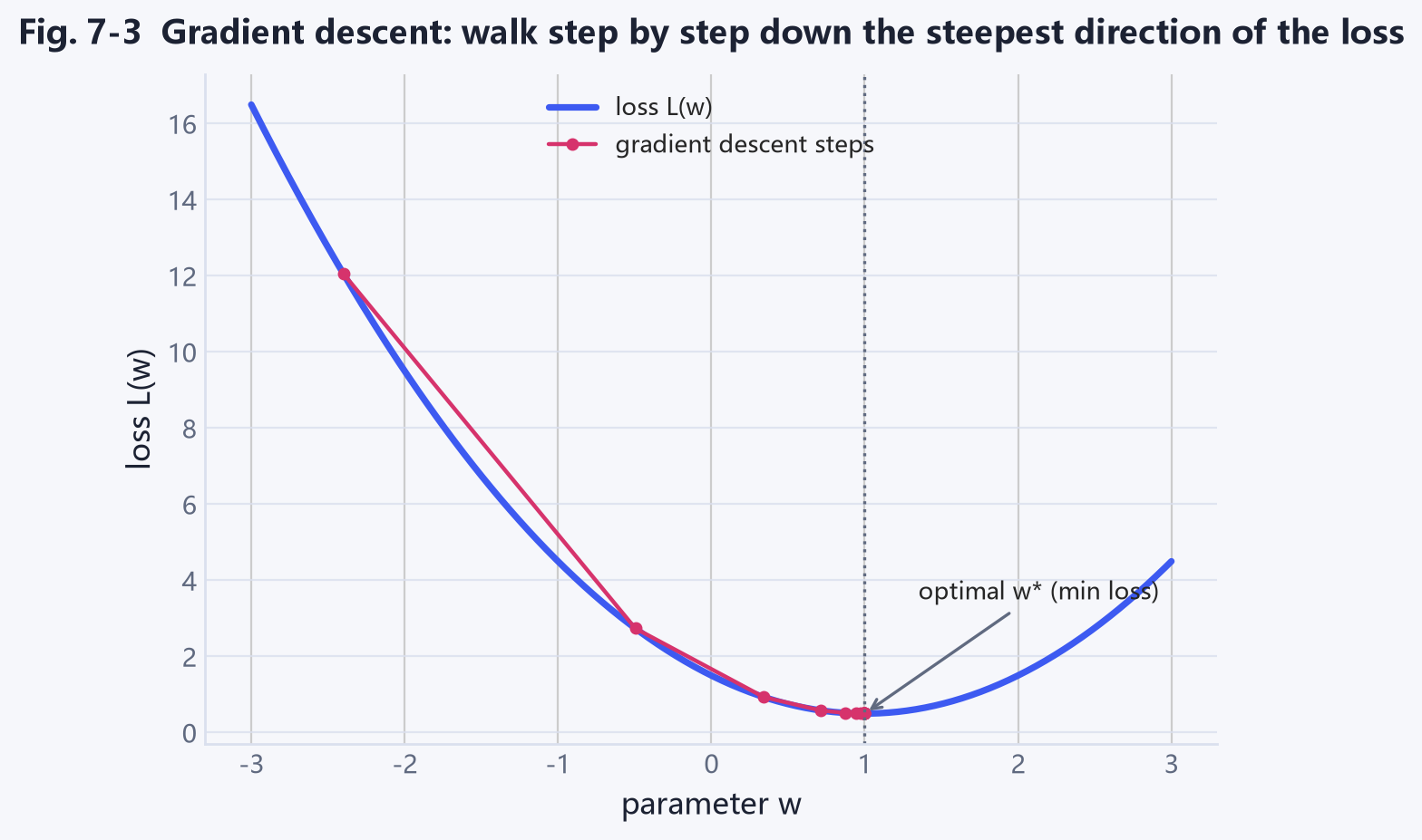
Fig. 7-3 (a simple “loss vs parameter” curve. The red staircase is gradient descent: start from the left and step down to the valley - the \(w^*\) where loss is smallest. The blue curve is the loss function, and the valley is the optimal parameter)
Tip | You absolutely do not need to derive the derivative. Remember three sentences: loss = how wrong the model is; training = find parameters that minimize loss; gradient descent = keep nudging in the direction that lowers loss fastest. scikit-learn wraps all this up for you.
7.5.1 Why Go Step by Step Instead of One Shot?#
In theory logistic regression’s loss is convex and has a closed-form solution. But in real projects:
With lots of data, inverting a big matrix is slow and unstable;
We want a method that generalizes to many models (trees, neural networks);
Gradient descent is the common engine for any model that minimizes a loss.
So understanding gradient descent means understanding how “training” works in linear, tree, and even neural models at once. That is its value.
7.5.2 An “anti-overfitting” dial: C and regularization#
If features are highly correlated or samples are few, the model may inflate weights to memorize the training data - a sign of overfitting. One defense is to add a penalty encouraging small weights (L2):
scikit-learn uses the inverse regularization \(C=1/\lambda\):
C=0.1-> \(\lambda=10\), strong regularization, weights sharply compressed, conservative;C=1.0-> \(\lambda=1\), moderate; largerCmeans less regularization.
Back to the code |
train_model.pyusesLogisticRegression(C=0.1)for base models (want them restrained, not memorizing), while the stacking meta-learner usesC=1.0(looser, freer to combine). Same class, two \(C\) - the trade-off “base models steady, meta-learner flexible.”
7.6 How Not to “Cheat”: Cross-Validation and Grouping#
Getting a high score on seen problems is easy; the real question is unseen problems. If a model memorizes the training samples, it collapses on new ones - overfitting.
The standard defense is cross-validation: cut the data into pieces and rotate which piece is the “mini-test”. But there is a trap easy to step into.
Watch out | One photo has 7 variants (1 clean + 6 hidden). They are too similar. If you split randomly, training could contain a “blood sibling” of some test photo - effectively telling the model the answer early. That is data leakage, and the score balloons unrealistically. The project’s fix: group by
photo_id- every variant of a photo is entirely in training or entirely in test, never split.
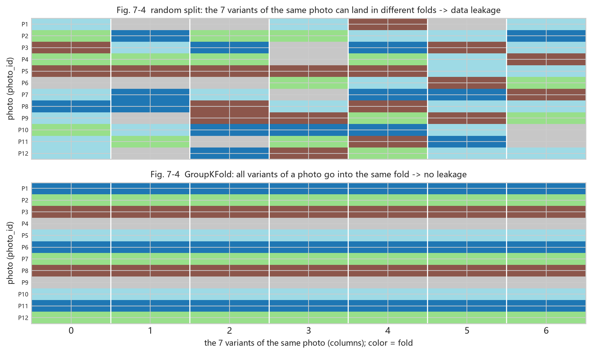
Fig. 7-4 (schematic: each P is a photo, one row has 7 variants. Top “random split” tears the 7 variants of a photo into different folds - leaks. Bottom “GroupKFold” puts all 7 variants of a photo into the same fold - honest)
Against the code - the core of src/train_model.py::cv_oof().
from sklearn.model_selection import GroupKFold
gkf = GroupKFold(n_splits=5)
for tr, va in gkf.split(X, y, groups):   # groups = photo_id, split by photo
    clf.fit(X[tr], y[tr])
    p = clf.predict_proba(X[va])[:, 1]   # score only on this "mini-test" fold
The key is the groups argument. It tells the splitter: “samples in the same group must not be torn apart.” The ordinary KFold would split a photo’s “blood siblings” across both sides, and the score would cheat.
Think about it | Why do the 7 variants of one photo not count as independent samples? Try a minimal example: with only 10 photos, how likely is a random split to put some photo’s “blood sibling” on both training and test sides? How much does such “leakage” inflate the score? (Hint: think about the 0.5 random line in 7.7.1)
7.7 Evaluation: Do Not Just Look at Accuracy#
The model outputs a probability, so we pick a threshold to say 0 or 1. For evaluating, start with the confusion matrix:
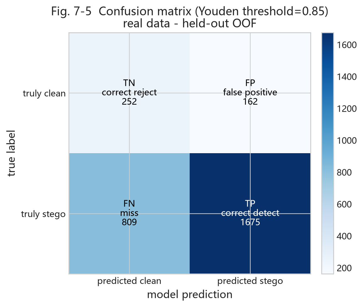
Fig. 7-5 (real data at the Youden threshold: TN = correct reject, FP = false positive, FN = miss, TP = correct detection. Numbers are real sample counts)
From these four values (TN, FP, FN, TP), the common metrics:
Accuracy: fraction correct overall. Trap: if there are far more hiding than clean, a model labeling everything “hiding” still scores high accuracy - but falsely accuses every clean image.
Precision: of those flagged hiding, how many really are.
Recall: of the truly hiding images, how many were caught.
F1: a compromise between precision and recall.
Metric |
Question it answers |
Intuition |
|---|---|---|
Accuracy |
How many right overall |
Misleading when imbalanced |
Precision |
Of flagged hiding, how many really are |
Low false-positives -> high |
Recall |
Of truly hiding, how many caught |
Low misses -> high |
F1 |
When you want both |
Compromise |
ROC / AUC |
Ranking strength, threshold-free |
0.5 = random |
7.7.1 ROC Curve and AUC: Can You Rank Hiding Above Clean?#
The key idea: a good model should rank hiding images above clean ones. Sweep the threshold from high to low and you get an ROC curve, horizontal = “false-positive rate”, vertical = “detection rate”. The closer to the top-left corner, the better.
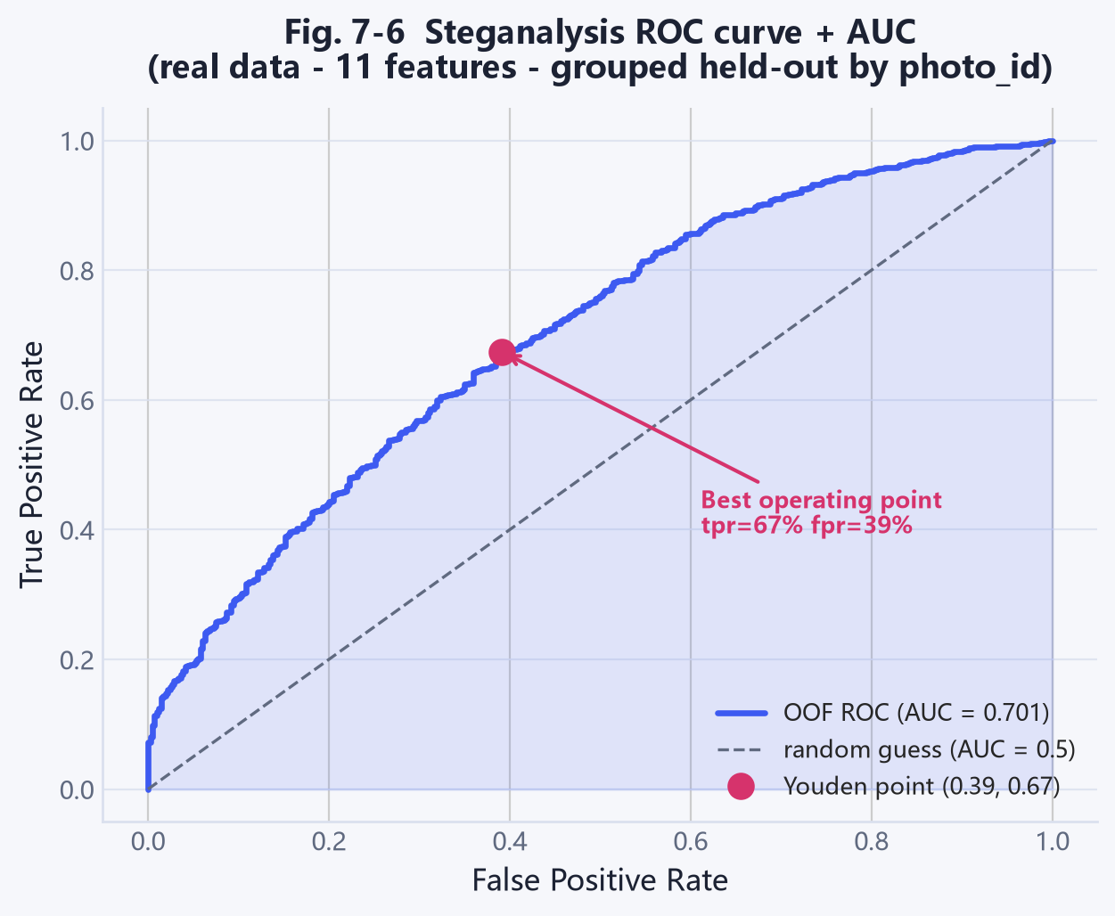
Fig. 7-6 (real-data OOF ROC curve: AUC ~0.70. The red shaded area is the AUC - “draw one hiding and one clean image at random; the probability the model ranks the hiding image higher.” The red dot is the Youden best operating point)
AUC is the area under the curve: 0.5 is random (diagonal dashed line), 1.0 perfect ranking. 0.7 means “usually ranks hiding above clean, but not great” - matching the reality that weak densities are hard to detect.
Key point | AUC is threshold-independent! No matter whether you set the threshold to 0.5 or 0.7, AUC stays the same. Because AUC only cares about ranking, not “where exactly to cut.” You can see this directly in Fig. 7-7.
7.7.2 Choosing a Threshold: The “Operating Point” on the ROC#
Although AUC is threshold-independent, in real deployment you must choose one. Higher -> conservative (fewer false positives, more misses); lower -> aggressive (more detection, more false positives). Look at this figure:
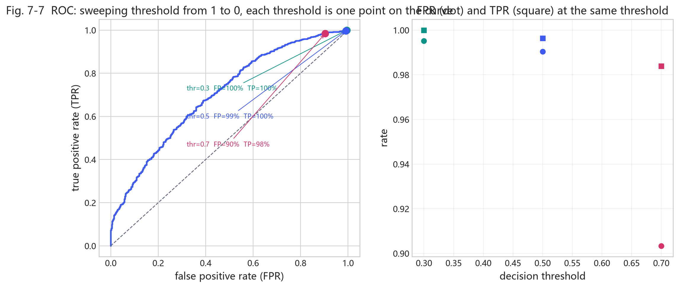
Fig. 7-7 (same test set. Left: thresholds 0.3/0.5/0.7 as three points on the ROC; Right: same thresholds’ detection rate TPR(■) and false-positive rate FPR(●). The lower the threshold, the higher the detection but also the higher the false positives - an unavoidable pair)
Back to the code |
train_model.pypicks the threshold with the Youden rule - the point maximizing “detection minus false-positive” (farthest from the random line), and also computes a low-FP threshold (FP<=10%) for strict mode:
from sklearn.metrics import roc_curve
fpr, tpr, th = roc_curve(y_true, proba)
j = tpr - fpr             # Youden J = detection - false-positive
best = float(th[np.argmax(j)])   # threshold with largest J, farthest from random line
7.7.3 Why “Accuracy” Misleads Here#
Imagine 2,484 of 2,898 samples are hiding: a model labeling everything hiding reaches accuracy \(2484/2898\approx85.7\%\), which looks great but false-positives all 414 clean images. So accuracy is meaningless under class imbalance; look at AUC, recall, and F1 instead.
I have drawn a figure showing exactly how each metric changes with the threshold:
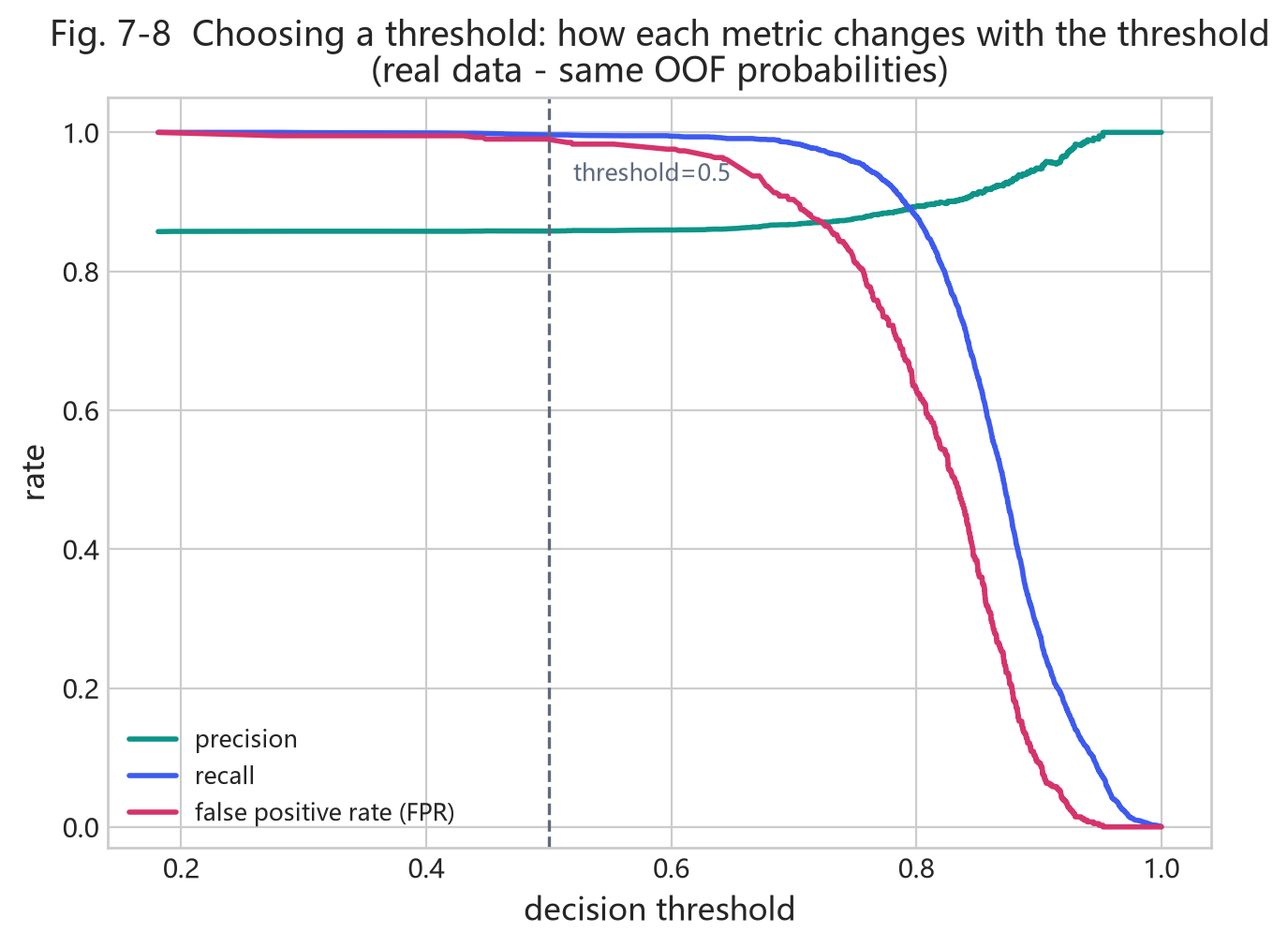
Fig. 7-8 (real data: as threshold falls from 1 to 0, precision (green), recall (blue), false-positive rate (red) change. Your chosen threshold is an “operating point” - a trade-off here)
Reading the figure:
Very low threshold: high recall (catch almost all), but low precision, high false-positive rate (over-flag clean images);
Very high threshold: high precision (flagged ones mostly real), but low recall (miss many);
Somewhere in between, you pick a “compromise point” that fits your need.
Try it | Run
python src\train_model.pyonce. You do not need to understand all output; first find three lines: CV-AUC, held-out test AUC, and low-FP detection rate. Chapter 8 explains them line by line.
7.8 Advanced: Two Bonus Bits in the Project (good to know roughly)#
train_model.py does two more things. On first read, just get the gist:
Probability calibration: logistic regression is often overly confident (says 0.95 when it should be 0.3). The project adds calibration so probabilities match real proportions, making thresholds meaningful.
Stacking: it does not bet on one model. It takes the answers of 4 models (logistic regression, random forest, gradient boosting, XGBoost) and lets a small model (logistic regression) learn “whose advice to follow”.
Tip | Stacking is like a jury: each juror (base model) scores independently, then a chairperson (meta-learner) combines the verdict. It does not pick one best; it merges the strengths of several ideas. Fig. 8-4 in Chapter 8 compares the four models side by side - then you see why they can “complement” each other.
7.9 Summary and Self-Check#
One sentence: machine learning = use “data -> features -> model -> evaluation” to turn “did this image hide something” into a judgeable, evaluable, explainable process.
Supervised learning = use “samples with answers” to learn a features-to-answer judgment;
Classification = separate two groups with a boundary; logistic regression = draw a line + sigmoid to probability (Fig. 7-1, 7-2);
Loss = points lost for wrong guesses; training = minimize loss; gradient descent = step downhill a little at a time (Fig. 7-3);
Do not randomly split same-source samples;
GroupKFoldgrouping byphoto_idis the honest way (Fig. 7-4);Accuracy distorts under imbalance; look at AUC / precision / recall; the threshold decides “strict or loose” (Fig. 7-5 ~ 7-8).
Think about it | A paper says “steganalysis AUC = 0.95” but never says how the data were split. What do you suspect first? Write it down - that is the start of evaluating every ML experiment. Go deeper: did it do calibration? How was its threshold chosen? Do these details also quietly cherry-pick a nice result?
Try it | After understanding Fig. 7-6 and 7-8, answer: if the boss demands “false positives must stay below 5%”, should you raise or lower the threshold? What is the cost?