Chapter 4 - Matrix Embedding and F5: Change Less, Hide More (Week 5)

🌐 中文版

Try it | Goals: understand why “embedding efficiency” matters; hand-compute a p=3 Hamming syndrome embedding example; read the matrix-coding schematic and efficiency curves; know F5’s “shrinkage” problem.

4.1 From “1 bit per pixel” to “p bits per change on average”

Naive LSB changes 0.5 pixels on average per stored bit - very inefficient. Suppose there were a code where each block of n pixels lets you store p bits by changing at most 1 pixel: changes drop dramatically. That idea is Matrix Embedding, and its math tool is the binary Hamming code.

Define embedding efficiency α = average bits carried per modification. The theoretical ceiling is p bits per change, α(p) = p·2ᵖ/(2ᵖ−1): ~2.67 at p=2, ~3.43 at p=3, ~4.27 at p=4, rising with p - but the block length n=2ᵖ−1 grows too.

Tip | Why is larger p “better”? Because the Hamming code uses n=2ᵖ−1 positions to carry p message bits; the bigger p, the less “waste” of n relative to p, and the more info each change carries on average. The cost: bigger blocks, and the message is pickier about the carrier structure. Look at Fig. 4-1 to see “7 positions hold 3 bits, flipping just 1 pixel” directly.

4.2 Hamming in a Nutshell: Parity-Check Matrix and Syndrome

Let block length n=2ᵖ−1. Build a p×n parity-check matrix H whose n columns are exactly all non-zero vectors in GF(2)ᵖ: at p=3 the seven columns are binary 1..7. Write the n pixel LSBs of a block as a column vector x, and define the syndrome s = H·x (mod 2), a p-bit vector.

To embed p message bits m, we want to flip a few bits so the new syndrome equals m. Since every column of H is distinct, flipping bit j only turns the syndrome into s⊕Hⱼ - that is, any needed syndrome change matches some column.

1. Compute the current syndrome s = H·x;

2. If s == m, no change needed in the block;

3. Otherwise compute the difference d = s ⊕ m (a non-zero p-bit vector);

4. Find the column of H equal to d - call it column j;

5. Flip the LSB of pixel j; done (H·x′ = m).

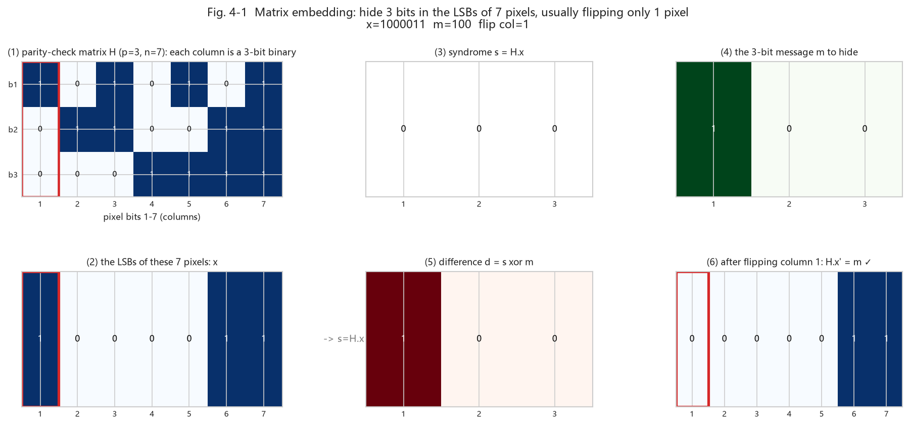
Fig. 4-1 (real computation: ① parity-check matrix H (p=3, n=7); the red box highlights the “target column”; ② this block’s 7 pixel LSBs: x; ③ current syndrome s=H·x; ④ the 3 message bits to hide: m; ⑤ difference d=s⊕m. Since d equals H’s column 1, only the 1st pixel’s LSB is flipped to get ⑥ the new syndrome = m)

Read this figure and you have all of matrix coding:

• H has 7 columns, each a 3-bit binary (for 1~7);

• s = H·x: XOR the columns where x is 1 to get the current syndrome;

• To turn the syndrome into m: just flip the pixel whose column equals d=s⊕m;

• Conclusion: to hide 3 bits, most cases only need 1 pixel changed.

4.3 A Worked p=3 Example

Let the 7 pixel LSBs of a block be x = [0,1,0,1,1,0,1]. Columns in binary order (low bit on top): H₁=[1,0,0], H₂=[0,1,0], H₃=[1,1,0], H₄=[0,0,1], and so on. First the syndrome: the 1-positions of x are columns 2,4,5,7; XOR them: H₂⊕H₄⊕H₅⊕H₇ = [0,1,0]⊕[0,0,1]⊕[1,0,1]⊕[1,1,1] = [0,0,1], so s=[0,0,1].

To embed m=[1,1,0]: d = s⊕m = [0,0,1]⊕[1,1,0] = [1,1,1]. H₇=[1,1,1], hits column 7, so flip the 7th pixel’s LSB: x′=[0,1,0,1,1,0,0]. Recompute s′=H·x′=[1,1,0]=m, success.

7 pixels carry 3 message bits, but on average only ~87.5% of blocks need a 1-bit change - about 0.875 changes per block, i.e. per 3 bits about 0.875 changes, ~3.43 bits per change.

Try it | src/matrix_demo.py turns this into a clickable visual panel (the “Matrix Coding Demo” tab in the GUI). Use demo_step(p, x, m_bin) to see the returned s, d, and the matched column, then verify H·x′ == m by hand.

4.4 Why Efficiency Matters: Capacity, Change Rate, and Detectability

“Hiding successfully” is not the skill; what matters is for the same message, the fewer changes, the smaller the statistical trace, the harder to detect. Let us plot the three quantities vs p with the real formulas - then you see the matrix-coding trade-off.

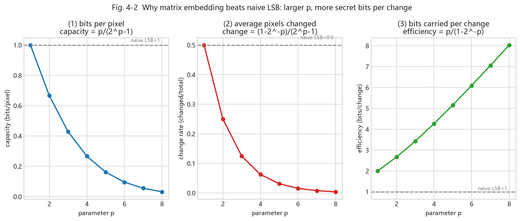
Fig. 4-2 (real computation: as p grows - ① capacity per pixel p/(2ᵖ−1) drops; ② average change rate (1−2⁻ᵖ)/(2ᵖ−1) drops sharply; ③ bits carried per change (embedding efficiency) p/(1−2⁻ᵖ) rises. Dashed lines are the naive-LSB baseline: capacity 1, change rate 0.5, efficiency 1)

Reading the figure:

• Change rate (②) directly measures “trace”: the larger p, the fewer pixels changed to hide the same message, the harder statistical detection catches it;

• Efficiency (③) measures “value per change”: p=3 is ~3.43 bits/change, over 3x naive LSB;

• Cost (①): the larger p, the smaller per-pixel capacity; hiding the same message needs a larger carrier.

Put them on one “capacity vs change-rate” trade-off plot and the trade-off is obvious:

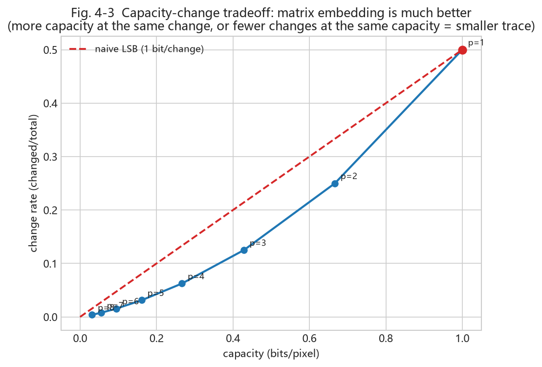
Fig. 4-3 (real computation: blue line is matrix coding at different p (capacity on x-axis, change rate on y-axis); red dashed line is naive LSB. The whole matrix-coding curve sits much lower - at the same change rate it hides more, or at the same capacity it changes less and leaves a smaller trace. That is why nsF5 in Chapter 5 insists on matrix embedding)

Tip | Steganography performance is usually measured by two things: capacity (how much) and distortion/change rate (how detectable). Matrix embedding’s meaning is to raise capacity at the same distortion, or lower distortion at the same capacity. This “change less = safer” idea runs through the nsF5 of Chapter 5 and the detection of Chapter 8.

4.5 F5: Matrix Embedding + JPEG Coefficient Decrement

F5 (Westfeld) is a JPEG steganographic scheme: it does matrix embedding on quantized DCT AC coefficients. Changing a “bit” is not an LSB flip but reducing the coefficient’s absolute value by 1 (e.g. +3→+2, −5→−4), which both flips the LSB parity and avoids obvious statistical anomalies.

The problem is “shrinkage”: when a coefficient with absolute value 1 is decremented, it becomes 0. A 0 coefficient in JPEG decoding means “no such frequency component”, so F5 treats it as no longer a legal carrier, drops the block, and retries later message bits. Shrinkage reduces the actual payload, lowers the achieved efficiency below the theory, and leaves a detectable statistical feature.

4.6 Back to the Project: MatrixEmbedding

Back to the code | Open the MatrixEmbedding class in src/ns5_core.py: _embed() is literally the 4.2/4.3 steps - compute s, compare m, find the column, flip. Fig. 4-1/4-2/4-3 are the visualizations of the math behind that code.

MatrixEmbedding._embed() core (real code excerpt)

xl = (c[pos] & 1).astype(np.uint8)     # take block LSBs
s  = syndrome(H, xl)                     # s = H·x
if np.array_equal(s, m): continue        # exactly matched, no change
d = (s ^ m).astype(np.uint8)             # difference
col = int(np.where(np.all(H == d[:, None], axis=0))[0][0])
c[pos[col]] ^= 1                         # flip the matched pixel

Back to the code | src/efficiency.py’s plot_code_family_and_efficiency() also draws the code family and efficiency plot (saved to output/efficiency.png), cross-checkable with Fig. 4-2.

4.7 Summary and Self-Check

• Matrix embedding works in blocks: n positions carry p bits, at most 1 change (Fig. 4-1);

• Distinct H columns ⇒ any syndrome difference locates the unique pixel to flip;

• Embedding efficiency α=p·2ᵖ/(2ᵖ−1), rising with p but block length grows too (Fig. 4-2);

• Capacity-change-rate trade-off: the fewer changes, the harder to detect (Fig. 4-3) - the fundamental answer to “why matrix coding”;

• F5 embeds by decrementing JPEG coefficients; shrinkage occurs when |coefficient|=1 becomes 0.

Think about it | If F5 skips and retries on shrinkage, can the message still decode correctly? How does the decoder know which blocks were skipped? Do not worry if stuck - Chapter 5’s nsF5 uses wet-paper coding to sidestep this entirely. One layer deeper: using Fig. 4-3, if I want to hide only 0.2 bit/pixel, how low can matrix coding push the change rate (versus naive LSB’s ~0.1)? That directly sets how hard steganalytic detection is.