Chapter 1 - Digital Images and Binary (Week 1)

🌐 中文版

Try it | Goals: cement the intuition that an image is a matrix of numbers; do binary and byte arithmetic by hand; explain why both the eye and statistics tolerate small pixel perturbations. We use the project’s real carrier (img/cover.png) to open up an image ourselves.

1.1 A Digital Image Is Just a Pile of Numbers

Zoom an 8-bit grayscale image down to the pixel level: it is a 2-D table of integers from 0 to 255. 0 is all black, 255 is all white, and between are shades of gray. The computer only stores the table’s “size” and “numbers”, not the picture your eye sees.

A color image is three such tables stacked: R (red), G (green), B (blue) channels. A common RGB image has 3 values (0-255) per pixel. For instance an orange pixel can be written R=255, G=128, B=0.

In code, a grayscale image is a 2-D array, and a color image is a 3-D array. The project’s src/image_io.py wraps this into two functions: load_as_gray() reads any supported image into a grayscale array, and save_image() saves an array to PNG.

Tip | Math uses “row, column” for matrices; image processing says “height, width”: a 512x512 image is 512 rows, 512 columns. The array shape (512, 512) is exactly “rows first”.

1.2 Binary, Bytes, and Bits

Computers only know 0 and 1. A single 0 or 1 is 1 bit; 8 bits make 1 byte. 8 bits can represent 2⁸=256 combinations, exactly matching gray values 0-255.

For example, decimal 200 = 128+64+8, written in 8-bit binary as 11001000; its least significant bit (LSB) is the rightmost 0. Change 200’s LSB to 1, and you get 201 - to the eye, gray 200 and 201 are nearly indistinguishable.

“Least significant bit” is one of the most important concepts in this whole handbook: LSB hiding is secretly modifying pixel LSBs to embed secret bits.

Try it | Open an interactive Python (or write a small script) and verify:

Experiment: decimal, binary, and LSB

v = 200
print(bin(v))            # 0b11001000
print(v & 1)             # lowest bit = 0
print(v ^ 1)             # flip lowest bit = 201
print(v & 0b11111110)    # clear lowest bit = 200
print(v & 0b11111110 | 1)# clear then set = 201

1.3 Why Images Have “Room” to Hide Things

Images contain lots of redundancy, understood at two levels:

• Visual redundancy: the eye is insensitive to tiny brightness differences and high-frequency detail. Changing a pixel from 128 to 129 is nearly invisible;

• Statistical redundancy: natural images have highly correlated neighboring pixels, with most information concentrated in low frequencies. JPEG compression shrinks files precisely by removing this redundancy;

• The LSB plane is near-random: the lowest bits of a natural photo look “like noise”, supplying a natural “cover environment”.

So two uses of redundancy appear: compression wants to remove redundancy to shrink the file, while steganography wants to stuff secrets into redundancy while disturbing visual/statistical features as little as possible. They fight over the same “modifiable space”, which is why many hiding algorithms are designed for specific compression formats.

Watch out | Do not think “invisible = safe”. Invisibility is only the weakest requirement; a professional detector uses statistics, and plain LSB replacement leaves a very obvious statistical trace - exactly what Chapter 3’s chi-square and RS analysis catch.

1.4 Bit Planes: Decompose an Image into 8 Layers

After writing gray values as 8-bit binary, you can decompose the image into 8 binary images by “which bit”, called bit planes. The most significant (MSB) plane determines the big outline; the LSB plane is almost all fine noise.

First, split the project’s real carrier (img/cover.png) by hand:

Fig. 1-1 (real data: far left is the original (0-255); the right 8 cells are bit 7 (MSB, x128) down to bit 0 (LSB, x1). Bit 7 decides the outline; bit 0 is almost all fine noise)

Reading the figure:

• The higher bit planes are the more “structured” (bit 7, 6, 5 resemble the original outline);

• The lower bit planes are the more “noise-like” (bit 0, 1, 2 full of random specks);

• Precisely because the LSB plane is already near-random, adding pseudo-random secret bits there is hard to notice visually or by a simple histogram - but statistics can tell it was “randomized” (Chapter 3).

Now do the “cumulative reconstruction” by hand too, to understand “each layer must be multiplied by its weight before adding”:

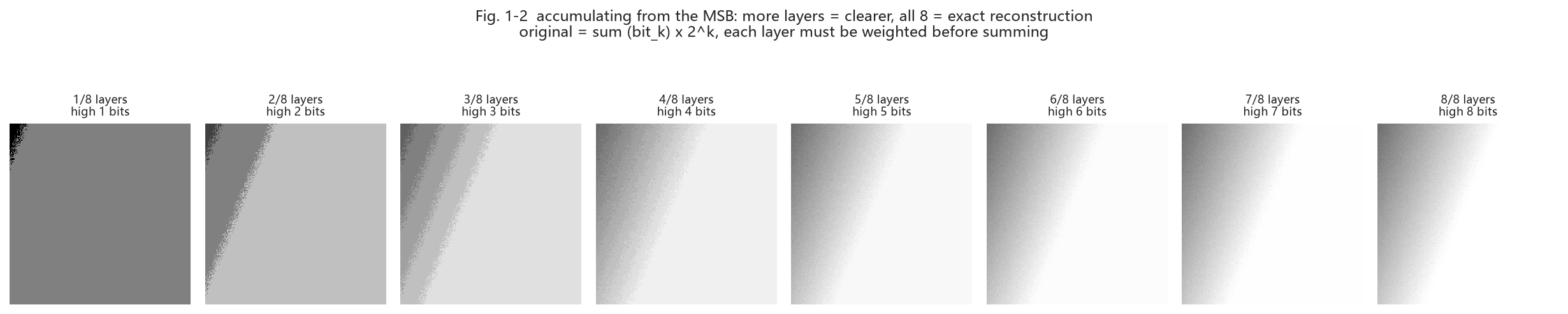
Fig. 1-2 (real data: accumulating from the MSB - first only bit7, a dark blocky outline; each added layer gets clearer; with all 8 layers it equals exactly the original)

This is the key sentence of “overlaying”:

\[ \text{original image} = \sum_{k=0}^{7} \text{bit plane}_k \times 2^{k} \]

A bit plane is only 0/1; it must be multiplied by its weight \(2^k\) before adding. If you just “OR” the 8 layers or add them ignoring weights, you do not get the original. That is why the project “changes LSB” with & 0xFE | bit (clear the LSB then set it) rather than integer add/subtract.

Tip | In Fig. 1-1 you see “high bits make the outline, low bits look like noise”. This intuition matters a lot: changing high bits = visible to the eye; changing low bits = invisible to the eye but measurable statistically. Hiding only touches the low bits, precisely because “low bits already look noisy, so changing them is not obvious” - both steganography’s opportunity and detection’s breakthrough.

Try it | Open the interactive lab (webapp/index.html) block 1 (bit-plane lab): pull out bit 0, bit 4, bit 7 individually and compare; switch to “cumulative reconstruction”, turn off bit 0, 1, 2 and watch the image go “flat”, then turn all 8 on to see it exactly recover the original.

Count pixels and LSB values (numpy operations you will see everywhere)

import numpy as np
img = np.asarray([[200, 201], [128, 129]], dtype=np.uint8)
print(img.shape, img.dtype)   # (2, 2) uint8
print(img & 1)                # LSB plane [[0,1],[0,1]]
print(np.unpackbits(np.array([200], dtype=np.uint8)))
# [1 1 0 0 1 0 0 0]  <- MSB first

1.5 Back to the Project: Meet cover and stego

Two fixed terms in this field: the original carrier without a secret is cover, and the image after hiding is stego. Both appear all over: img/cover.png is the demo carrier, and output/stego_*.png are the embedded images.

Back to the code | Open step 1 of src/run_e2e.py: it uses numpy to generate a 256x256 smooth “cover” and saves it to img/cover.png. Look closely - np.linspace makes the gradient background, then a little noise is added. Understanding this code shows how a natural-looking image “grows” out of numbers. (Fig. 1-1/1-2 use exactly this image.)

1.6 Summary and Self-Check

• A grayscale image = a matrix of 0-255 integers; a color image = three channel matrices;

• The LSB is the lowest bit of a pixel’s binary value; flipping it has a tiny visual effect (Fig. 1-1);

• Compression removes redundancy; steganography uses it; they are at odds;

• cover = original carrier, stego = the image with a secret;

• High bits make the outline, low bits look like noise - the root of “hiding in low bits, detection measuring low bits” (Fig. 1-2).

Think about it | Is a pure black (all 0) image a good LSB carrier? What about a pure random-noise image? Write it down, then come back after Chapter 3. (Hint: whether the LSB plane is “near-random” decides both how easy it is to hide and how easy it is to catch.)