Chapter 3 - LSB Steganography and Its Statistical Fingerprint (Weeks 3-4)

🌐 中文版

Try it | Goals: complete the smallest possible “hide then detect” loop; understand what chi-square and RS analysis each measure; read the verdict logic in steganalysis.py. First we visually see how “subtle” an LSB change is on a real carrier (img/cover.png), then see how statistics expose it.

3.1 Encryption vs Steganography: The First Question

Aspect	Encryption	Steganography
Protects	Message content: unreadable without a key	Communication: nobody sees there is a secret
Visibility	Ciphertext clearly “not normal data”	Carrier looks completely normal
Typical use	Passwords, certificates, encrypted files	Covert channels, watermarking, forensics
Relation	Can encrypt then hide (recommended)	Steganography hides the “existence” of a secret

Tip | A one-line rule: encryption protects “content”, steganography protects “existence”. Professional systems usually use both: encrypt the message first, then hide the ciphertext. Encrypted ciphertext looks near-random, which is less likely to reveal itself statistically.

3.2 Minimal Runable LSB Steganography

The simplest steganography is LSB replacement: write the secret bit string into the LSBs of pixels one by one. A grayscale image with M×N pixels can hide M×N bits.

Textbook minimal LSB (for understanding only; the project actually uses matrix coding from Chapters 4-5)

import numpy as np
 
def text_to_bits(s):
    raw = s.encode("ascii")
    # 16-bit length header + 8 bits per character
    head = [(len(raw) >> i) & 1 for i in range(16)]
    body = np.unpackbits(np.frombuffer(raw, np.uint8))
    return np.concatenate([head, body]).astype(np.uint8)
 
def lsb_embed(cover, bits):
    flat = cover.ravel().copy()
    k = min(len(bits), flat.size)
    flat[:k] = (flat[:k] & 0xFE) | bits[:k]   # clear LSB then write
    return flat.reshape(cover.shape)
 
def lsb_extract(stego, nbytes):
    flat = stego.ravel() & 1
    return bytes(np.packbits(flat[16:16 + nbytes*8]))

Watch out | Lossy formats are LSB’s enemy. PNG/BMP losslessly preserve bit planes; JPEG compression destroys LSBs. So the project saves PNG by default, and JPEG-domain hiding needs a separate route (the companion project yccstego goes the quantized-DCT-coefficient route; it is a separate repository and PyPI package, not part of this repository).

Why put a 16-bit length header first? Because the decoder must know “how many bytes to read” to recover the message. The project’s encode_string() in src/ns5_core.py writes a 16-bit little-endian length first, then the ASCII body bits - you have replicated that structure in the 3.2 example.

3.2.1 First, See It: How “Subtle” Is an LSB Change?

On the project’s demo carrier img/cover.png, do one real LSB replacement (hide random bits) - about 25% of pixels have their LSB rewritten. See what the image becomes:

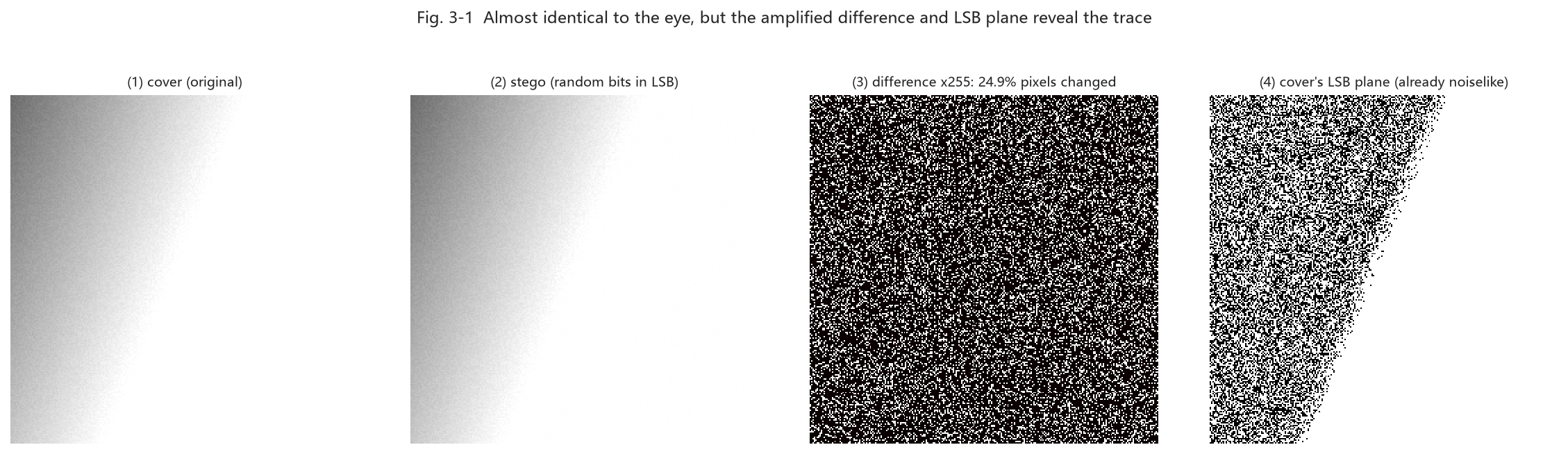
Fig. 3-1 (real data: ① carrier img/cover.png; ② stego after hiding random bits via naive LSB; ③ amplify |cover − stego| ×255 to finally see the changes scattered across the image; ④ the carrier’s own LSB plane - already near-noise)

Reading the figure:

• ① vs ② look identical to the eye - that is LSB’s “concealment”;

• ③ amplified ×255 reveals the noise scattered over the image - the “positions of changed pixels”;

• ④ cover’s LSB plane is already fine noise - so adding random bits there is hard to notice visually or by histogram.

3.2.2 Pixel Level: How Many Changed, and How?

Zoom into a small real block of pixel values and see each pixel’s change before/after:

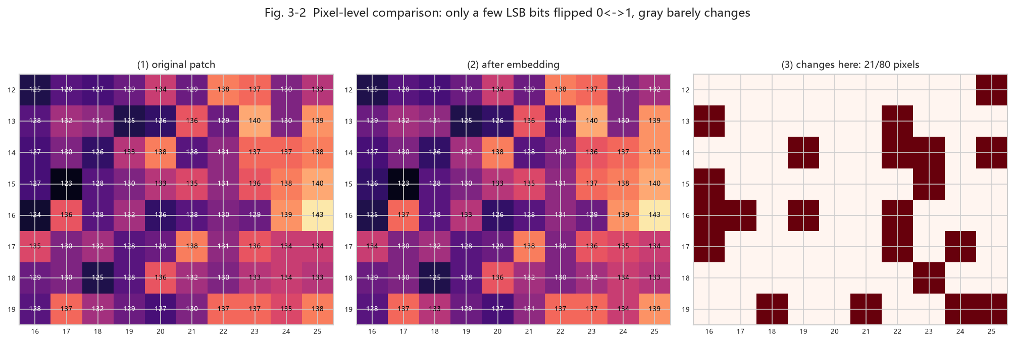
Fig. 3-2 (real data: ①/② the same small region’s gray values before/after embedding; ③ marks the 21/80 pixels changed. Note every change differs by only 1 - because only the LSB flips 0↔1)

Reading the figure:

• Each changed pixel’s value moves by only ±1 (e.g. 127→128, 135→134), because only the lowest bit changes;

• The eye is completely insensitive to a 1-level gray change - that is “visual redundancy”;

• But exactly this “pair-flattening” change leaves a measurable fingerprint for statistical detection (3.3 chi-square, 3.4 RS).

Tip | Remember two words: visual redundancy (the eye cannot see) and statistical redundancy (a detector can see). LSB hiding uses the former but breaks the latter - that becomes the breakthrough for all statistical detection.

3.3 Why It Is Exposed: The Chi-Square Test

In natural images the adjacent gray values 2i and 2i+1 (e.g. 100 and 101) usually appear with unequal counts. LSB replacement forces the even/odd pair to “flatten”: when a pixel changes from 2i to 2i+1 or back, the two gray counts tend to equalize. Westfeld’s chi-square test does exactly this:

1. Count the 256-level grayscale histogram and pair adjacent values (0,1),(2,3),…,(254,255);

2. Assuming “embedded”, the two counts in each pair should be nearly equal; the expected value is half the pair sum;

3. Compute Σ(observed−expected)²/expected (only over pairs with positive count);

4. Convert to a p-value: high p means “consistent with the uniform assumption” → suspect LSB randomization;

5. The project also cuts the image into 20 prefix segments, computes a p per segment, and takes the median for a steadier verdict.

Note the p-value meaning is easy to get backwards: here a larger p is more suspicious, because it says “if the LSB were fully randomized, seeing this distribution is likely” - a clean smooth image usually is not so uniform.

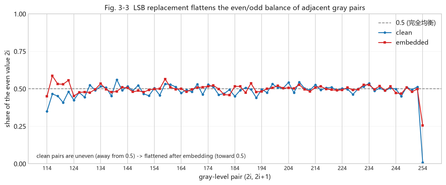
This compares, for each adjacent gray pair (2i, 2i+1), the proportion of pixels that take the even value for a clean image and after LSB embedding: the clean image (blue) clearly deviates from 0.5 (uneven even/odd counts); after embedding (pink) it is “flattened” toward 0.5. That is exactly the signal chi-square catches - the more balanced, the higher the p, the more suspicious.

Watch out | A naturally noisy image can fool chi-square. Digital photos already have near-random LSBs, so the chi-square p is naturally high. So the project adds a “content randomness” correction: first estimate how random the image inherently is via the grayscale difference entropy, then decide whether to treat a high p as evidence of embedding. This is a key engineering detail that makes the heuristic usable.

3.4 RS Analysis: The “Structural Collapse” of the LSB

Fridrich et al.’s RS analysis takes a different angle: instead of comparing gray-pair counts, it looks at the spatial structure of the LSB plane. It cuts the pixel stream into groups of 4, defines a smoothness discriminant f (sum of absolute adjacent differences within the group), then uses a “positive mask” and “negative mask” to flip some LSBs in the group, counting groups where f increases (Regular R) or decreases (Singular S) after flipping.

A clean natural image has a clear “regular tendency” under the negative mask, quantified by Gn = (Rn−Sn)/N which is clearly positive (the project’s clean smooth images often 0.3-0.7). LSB replacement randomizes the plane, collapsing this structure - Gn drops markedly. The project also reports Gr, estimated embedding rate, etc., together forming the “RS evidence”.

The core RS logic in the project’s steganalysis.py (pseudocode, only illustrating the grouping/statistical idea)

groups = flat[:m].reshape(-1, 4)        # group of 4 pixels
fg = np.abs(np.diff(groups, axis=1)).sum(axis=1)   # original smoothness f
pos = (groups ^ np.array([0,1,1,0])) & 0xFF        # +M flip
neg = (groups ^ np.array([1,0,0,1])) & 0xFF        # -M flip
Rm = (f(pos) > fg).sum();  Sm = (f(pos) < fg).sum()
Rn = (f(neg) > fg).sum();  Sn = (f(neg) < fg).sum()
Gn = (Rn - Sn) / n          # clearly positive for clean, ~0 after randomization

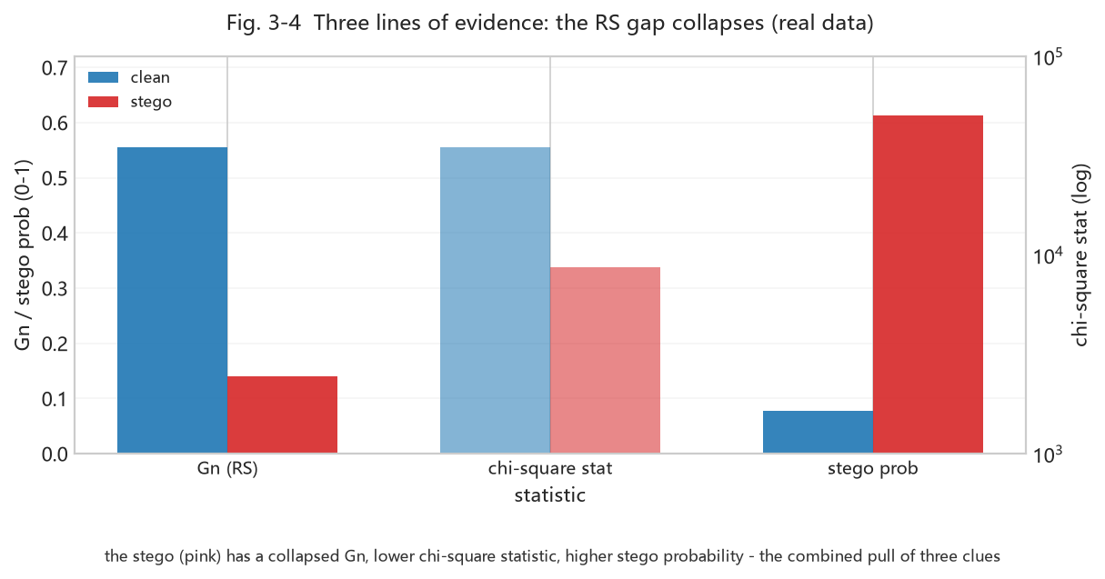
This uses the project’s real statistics to compare clean (blue) vs stego (pink): the RS gap Gn collapses from clearly positive (structure), the chi-square statistic drops (even/odd gets flattened), and the ML stego probability rises. LSB embedding destroys the LSB plane’s “order” - this bar chart is a direct comparison of the three lines of evidence (RS / chi-square / ML).

3.5 The Project’s Combined Verdict: analyze()

src/steganalysis.py’s analyze(image, sensitivity=...) does not look at one statistic, but combines four signals:

• median chi-square p (are gray pairs flattened?);

• RS collapse amplitude (how far Gn drops relative to a content-adaptive baseline);

• grayscale difference entropy and LSB difference entropy (is the randomness native to the image?);

• the prefix p sequence (is the randomization local or global?).

Three sensitivity levels (strict / balanced / loose) tune the “possible / highly possible” thresholds and the probability-pull coefficient, essentially choosing an operating point between false positives and misses.

Look ahead to Chapter 7 | Chapter 7 upgrades this heuristic into “features + a supervised classifier” and draws fuller ROC / AUC (Fig. 7-6) and feature distributions (Fig. 8-1/8-2).

3.6 Hands-On: Hide a Sentence, Then Catch It

Using the real project API: embed -> save -> analyze (run cell by cell in Jupyter)

import sys; sys.path.insert(0, "src")
import numpy as np
import image_io as IO
from ns5_core import embed_string, extract_string
import steganalysis as SA
 
clean = IO.load_as_gray("img/cover.png")
stego, report, nbits = embed_string(
    clean, "Hello nsF5!", method="nsF5", p=3, password="")
import os; os.makedirs("output", exist_ok=True)   # repo convention: script outputs go here
IO.save_image(stego, "output/lab3_stego.png")
print("changed pixels:", report["cover_changed"])
print("decoded:", extract_string(stego, method="nsF5", p=3))
for name, im in (("clean", clean), ("stego", stego)):
    r = SA.analyze(im)
    print(name, "Gn=%.3f" % r["RS_Gn"],
          "chi2p=%.3f" % r["chi2_pvalue"],
          "prob=%.2f" % r["stego_probability"], r["verdict"])

Try it | Change the message to 5000 characters and run again (see src/test_steg.py); watch the changed-pixel ratio, Gn drop, and stego probability change. Then swap in a noisier photo and see whether chi-square and RS can still distinguish.

3.7 Summary and Self-Check

• LSB embedding uses visual redundancy (Fig. 3-2: each change differs by 1), invisible to the eye (Fig. 3-1);

• LSB replacement flattens adjacent gray-pair counts (chi-square) and destroys LSB-plane structure (RS);

• A high p is not “safe”; first judge whether the image is naturally random;

• False positives vs misses are a trade-off; the sensitivity setting picks an operating point;

• The project’s analyze() is an engineering combination of “statistical signals + content baseline”.

Think about it | Plain LSB replacement hides 1 bit/pixel with an average 50% change rate. If you hide only a small message and change less than 1% of pixels, can chi-square still catch it? RS? Take this question into Chapter 4. One layer deeper: Fig. 3-1 shows the LSB plane is already near-noise - so why does chi-square still catch it? (Hint: the key is “a clean image’s even/odd counts are initially uneven”, not “the LSB looks random”.)