Chapter 8 - Machine-Learning Steganalysis (Weeks 8-14)

Chapter 8 - Machine-Learning Steganalysis (Weeks 8-14)#

🌐 中文版

Try it | Goals: understand why features instead of raw pixels; recognize what each of the 11 features measures (with real distribution figures); read 4 classifiers and 4 real ROC curves; run the full “generate data -> train -> judge” flow. Section 8.8 covers the complete v1.4 evolution.

8.0 Chapter Roadmap (about 4-8 weeks)#

Step 1 (~1 week): 8.1, understand “why features instead of a raw CNN” - the most important step in this book; make sure you get it.
Step 2 (~2 weeks): 8.2, meet the 11 features one by one. Use Fig. 8-1/8-2 distributions, cross-check formulas and steganalysis.py.
Step 3 (~2 weeks): 8.3-8.4, understand “where data come from + how to read the training script”. Use Fig. 8-3/8-4.
Step 4 (~2 weeks): 8.5-8.7, learn to read ROC / detection rates and run the full pipeline.
Step 5 (advanced, ~1 week): 8.8 v1.4 evolution (SRM, 143-D, dual models) - the part closest to a paper.

8.1 A Counterintuitive Question: Why Not Just Let the AI “Look”?#

You heard deep learning can recognize cats and dogs. Why not feed raw pixels to a network and let it learn “hidden or not” by itself? The project tried - validation AUC ~0.50, essentially random guessing. The reasons:

Steganography changes an extremely weak high-frequency signal (the LSB layer), far weaker than image content or texture;
A network easily learns “this is a landscape, that is a portrait” rather than “hidden or not”;
The number of truly independent samples is the number of photos (hundreds), while deep models usually need thousands.

So the project took another path: use human domain knowledge to measure the statistical traces hiding leaves (features), then let a simple classifier judge. v1 used 11 features with AUC ~0.75-0.79 on small data; v1.4 raised it to 0.90+ with 143-D features and LightGBM (see 8.8), but “features beat raw CNN” still holds.

Tip | This is not “deep learning is useless”, but a lesson in how to choose a method when data are scarce: first verify the signal with strong explainable features, then consider a more complex model. Many engineering problems follow the same order.

8.2 Meet the 11 Features: What Are They Measuring?#

The v1 features come from the C++ library cpp/fsfeatures.dll (Python wrapper in src/fsfeatures.py); the 143-D v2 set is built in src/featurize_v2.py. First, one big impression: these 11 numbers are 11 rulers, each measuring “was the LSB plane messed with”. They fall into three groups:

Feature	Measures	After hiding
Rm / Sm / Gr	Regular/singular counts and gap under +M	Gr drops
Rn / Sn / Gn	Counts and gap under -M	Gn collapses (core signal)
chi2_stat / chi2_pvalue	Were gray pairs “flattened”?	Pairs balance, p rises
diff_entropy	Native texture roughness	Used to spot naturally noisy images
lsb_diff_entropy	Is the LSB plane chaotic?	Approaches 1 when randomized
median_prefix_p	Median chi-square p over 20 prefixes	Rises when globally randomized

Now the “skill” of each ruler. Look at the distribution figures first, then the formulas - figures are more intuitive.

8.2.1 RS Analysis: Where the Core Signal Gn Comes From#

RS (Regular-Singular) groups pixels 4 at a time $g=(g_1,g_2,g_3,g_4)$ and defines “how smooth this group is” using the sum of adjacent differences:

\[ f(g)=|g_1-g_2|+|g_2-g_3|+|g_3-g_4| . \]

Pick a mask $M=(0,1,1,0)$, flip LSBs at certain positions to get a new smoothness $f_M$; its complement is the negative mask. Each group is then:

Regular: after flip $f_M > f$ (smoother/regular);
Singular: after flip $f_M < f$ (messier).

Then the gap is the difference of the two counts as a fraction of the total:

\[ G_r=\frac{R_M-S_M}{n},\qquad G_n=\frac{R_{-M}-S_{-M}}{n}. \]

Fig. 8-1 RS feature distributions

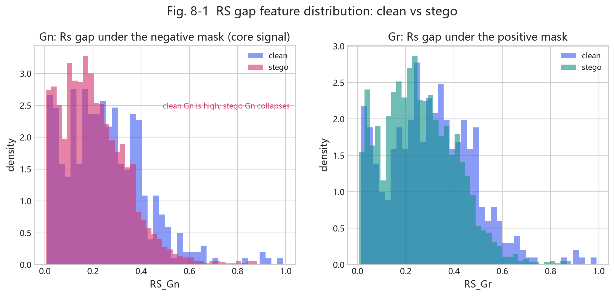
Fig. 8-1 (real data: RS gap distributions for clean (blue) and hiding (red). Left: Gn (negative mask) - clean images cluster higher while hiding collapses toward low values; that is the strongest signal. Right: Gr (positive mask) also separates, but less cleanly than Gn)

In plain words: a clean image’s LSB plane has structure (adjacent LSBs often correlate). Flip the negative mask and many groups go from regular to singular, so $G_n$ is clearly positive (0.3-0.7 on clean images). After hiding, the LSB plane is randomized, the two masks behave alike, and $G_n$ collapses toward 0. So Gn collapse = strong evidence of hiding.

Against the code - src/steganalysis.py::rs_metrics.

gi = groups.astype(np.int16)                     # group of 4 pixels
fg = np.abs(np.diff(gi, axis=1)).sum(axis=1)     # f(g) = Σ|adjacent diff|
pos = ((gi ^ mask) & 0xFF)                        # group after positive-mask flip
fM  = np.abs(np.diff(pos, axis=1)).sum(axis=1)
Rm = int(np.sum(fM > fg)); Sm = int(np.sum(fM < fg))
# finally {"Gr": (Rm - Sm) / n, "Gn": (Rn - Sn) / n}

8.2.2 Chi-Square Test: Were Gray Pairs “Flattened”?#

Westfeld pairs gray values $(2i,\,2i+1)$. In a clean image these two gray frequencies usually differ; LSB randomization flattens them. The chi-square measures deviation from uniform:

\[ \chi^2=\sum_i \frac{(O_i-E_i)^2}{E_i},\qquad O_i=\text{observed even-gray frequency},\ E_i=\frac{f_{2i}+f_{2i+1}}{2}. \]

The p-value comes from an incomplete gamma: $p=Q(df/2,\ \chi^2/2)$, with degrees of freedom $df=$ (active pairs - 1).

In plain words: a high p-value means the observation is barely different from “perfectly even” - that gray pair has already been randomized/hidden.

A small detail (nice to know): the code writes (even-odd)²/(even+odd), exactly twice the textbook formula. Since it just multiplies each term by a constant, the ranking of “which image is more suspicious” is unchanged - only the p-value scale differs.

Against the code - steganalysis.py::chi2_stats and _prefix20_p.

even = counts[0::2]; odd = counts[1::2]
stat = float(np.sum((even[mask]-odd[mask])**2 / sums[mask]))   # chi-square
return stat, float(chi2_sf(stat, n-1)), n-1                    # chi-square, p, df

Back to the code | median_prefix_p cuts the image into 20 prefixes, computes a p-value per prefix, and takes the median - so a single segment’s fluke does not sway the judgement.

8.2.3 Entropy: How Naturally Chaotic Is the Image?#

The Shannon entropy of adjacent-pixel absolute differences measures the image’s native chaos:

\[ H=-\sum_{d=0}^{255} p(d)\log_2 p(d),\qquad p(d)=\frac{\#\{\text{adjacent abs diff}=d\}}{\text{total pairs}} . \]

diff_entropy: entropy over grayscale differences. Smooth/structured images low (~1-3), high-noise/dithered near 8.
lsb_diff_entropy: keep only the LSB plane (pixel & 1), then entropy over adjacent differences, range 0-1. Fully random LSB -> 1, clearly structured -> <0.7.

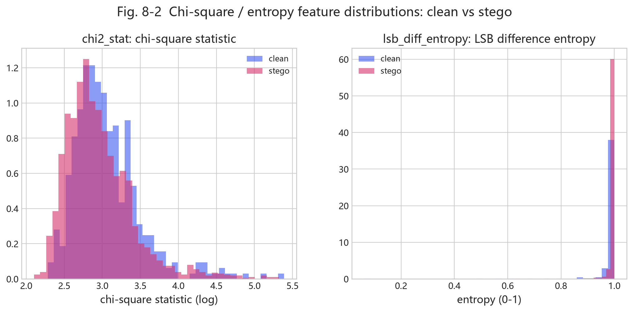
Fig. 8-2 chi-square/entropy feature distributions

Fig. 8-2 (real data: Left: chi-square statistic (log) - clean (blue) is higher (even/odd more uneven), hiding (red) lower (more “flattened”). Right: LSB difference entropy - hiding (red) toward 1 (LSB more random), clean (blue) lower)

In plain words: these two features recognize images that are naturally messy (high-noise photos, dithering) so we do not misjudge them as hiding - they backstop “can we even conclude reliably”. For example, an image with lsb_diff_entropy very close to 1 could be natural noise or could be hiding; cross-check with other features.

8.3 Where Data Come From: The “1+6” Design of make_dataset.py#

Training data cannot come from hand-hiding a few messages. src/make_dataset.py produces one clean image plus six hiding variants per source photo (v1.4 supports 12; see 8.8):

Variant (method, p, density)	Strength	Purpose
clean	-	Clean negative samples
nsF5, p=3, d=0.25	weak	Close to realistic covert communication
nsF5, p=3, d=0.55	medium	Moderate strength
nsF5, p=2, d=0.35	weak-medium	Lower p is less efficient, leaves more traces
nsF5, p=2, d=0.85	strong	Heavy embedding, obvious footprint
matrix, p=3, d=0.50	medium	Compare another method
matrix, p=2, d=0.80	strong	High-density plain matrix embedding
v1.4 adds +6	-	nsF5 p3 d0.40; matrix p3 d0.40/0.60; lsb d0.30/0.50/0.70

All images resize to 512x512 grayscale; features come from C++ and hiding variants are produced by the C++ embedding path, so training and inference stay consistent.

Tip | The “p, density” on the right is exactly the “embedding strength” from 8.1: the stronger the band, the more is hidden, the clearer the statistical trace, the easier the classifier. That is also why weak densities are harder to detect (Fig. 8-5).

8.4 How to Read the Training Script: train_model.py#

python src\train_model.py is one honest evaluation pipeline:

Load the table and drop rows with missing features;
Reserve 25% as the final test set by photo_id (those photos never enter training);
On the training pool, run 5-fold cross-validation comparing logistic regression / random forest / gradient boosting / XGBoost;
Pick the best CV model, carve 20% of the training pool as a calibration set, and choose a threshold;
Retrain on the full training pool and report AUC / accuracy on the held-out test set;
Report per-(method, p, density) detection rates;
Save the model and thresholds to models/stego_classifier.joblib.

8.4.1 Four Classifiers, Each an Approach (ideas + real comparison)#

Step 3 compares four models - really just three ideas:

Logistic regression (LR): the “draw a line + sigmoid to probability” from Chapter 7. Most intuitive, most stable, most explainable; con: the line is straight, it cannot bend.
Random forest (RF): a crowd of trees voting. Each tree asks a chain of “if this feature > some value, go left, else right.” Many trees trained on different samples and features, then majority vote. Stable, resists overfitting.
Gradient boosting / XGBoost (GB/XGB): relay to fix errors. Not many trees at once - one after another, each tree fixes what the previous got wrong. XGBoost is the “upgraded” version with extra anti-overfitting rules: fast, often best.

def lr(seed=0):  return make_pipeline(StandardScaler(), LogisticRegression(max_iter=2000, C=0.1, random_state=seed))
def rf(seed=0):  return RandomForestClassifier(n_estimators=500, max_depth=None, min_samples_split=2, n_jobs=-1, random_state=seed)
def gb(seed=0):  return GradientBoostingClassifier(n_estimators=300, learning_rate=0.05, max_depth=3, random_state=seed)
def xg(seed=0):  return XGBClassifier(n_estimators=400, learning_rate=0.05, max_depth=4,
                    subsample=0.9, colsample_bytree=0.8, eval_metric="logloss", random_state=seed, n_jobs=-1)

Fig. 8-4 classifier ROC comparison

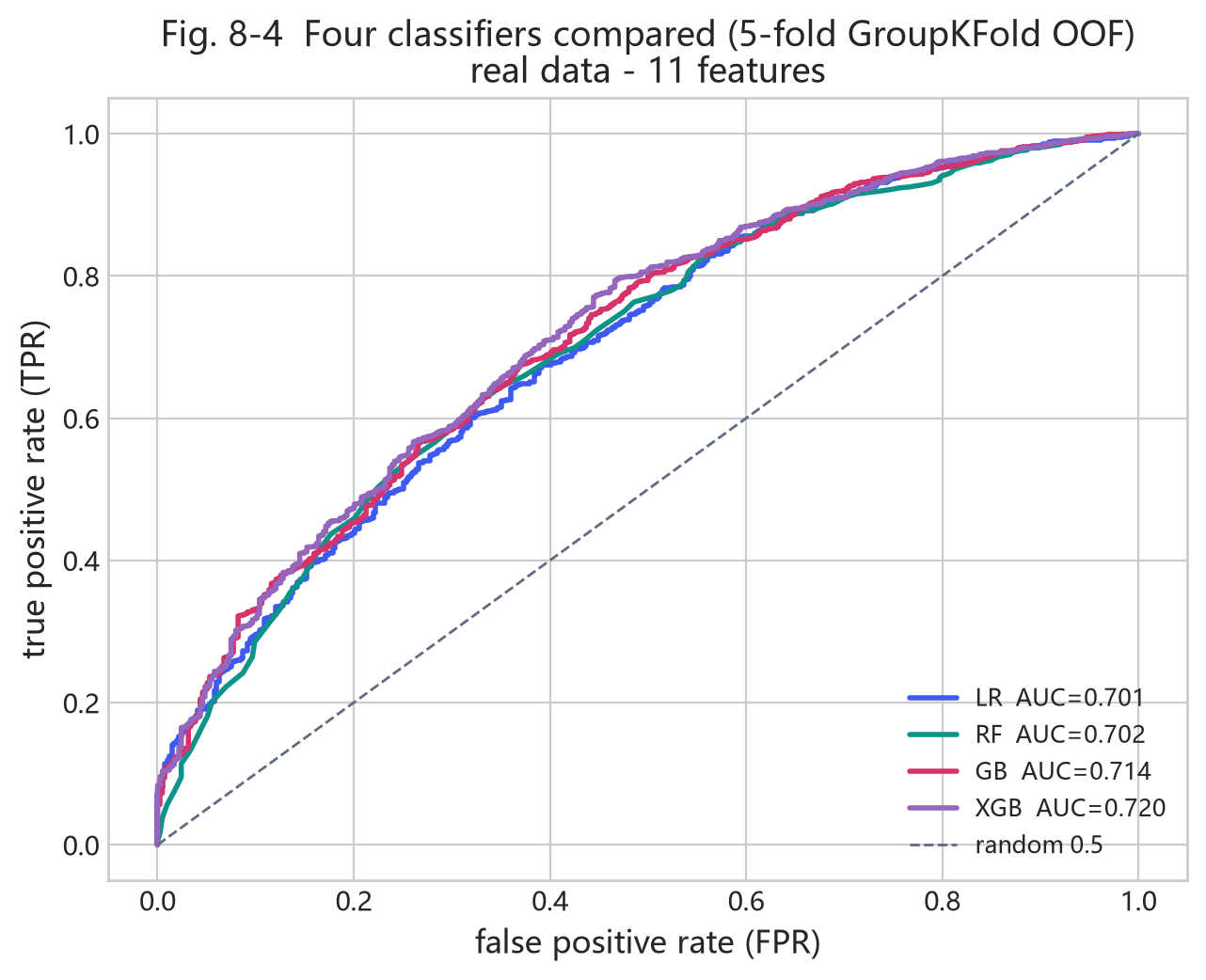
Fig. 8-4 (real data 11-D, 5-fold GroupKFold OOF: the four classifiers’ ROC curves nearly overlap, all AUC between 0.70-0.72. This means on these 11-D features the method matters little - the bottleneck is more in the features than the classifier, which backs up 8.1: get the features right first, then pick a classifier)

If you want to go deeper | A tree splits by picking one feature and one threshold that splits samples into two piles, each as “pure” as possible. Purity uses Gini impurity $G=1-\sum_c p_c^2$ or information entropy. n_estimators=500 means plant 500 trees; learning_rate=0.05 is “step gently”. No need to memorize - just know “trees split toward purity” and “XGBoost is more restrained.”

8.4.2 Which Feature Matters More: Look at the LR Coefficients#

Since the classifiers differ little, the features are what matter. The weights $w$ learned by logistic regression directly tell us how much each feature contributes and in which direction:

Fig. 8-3 feature importance

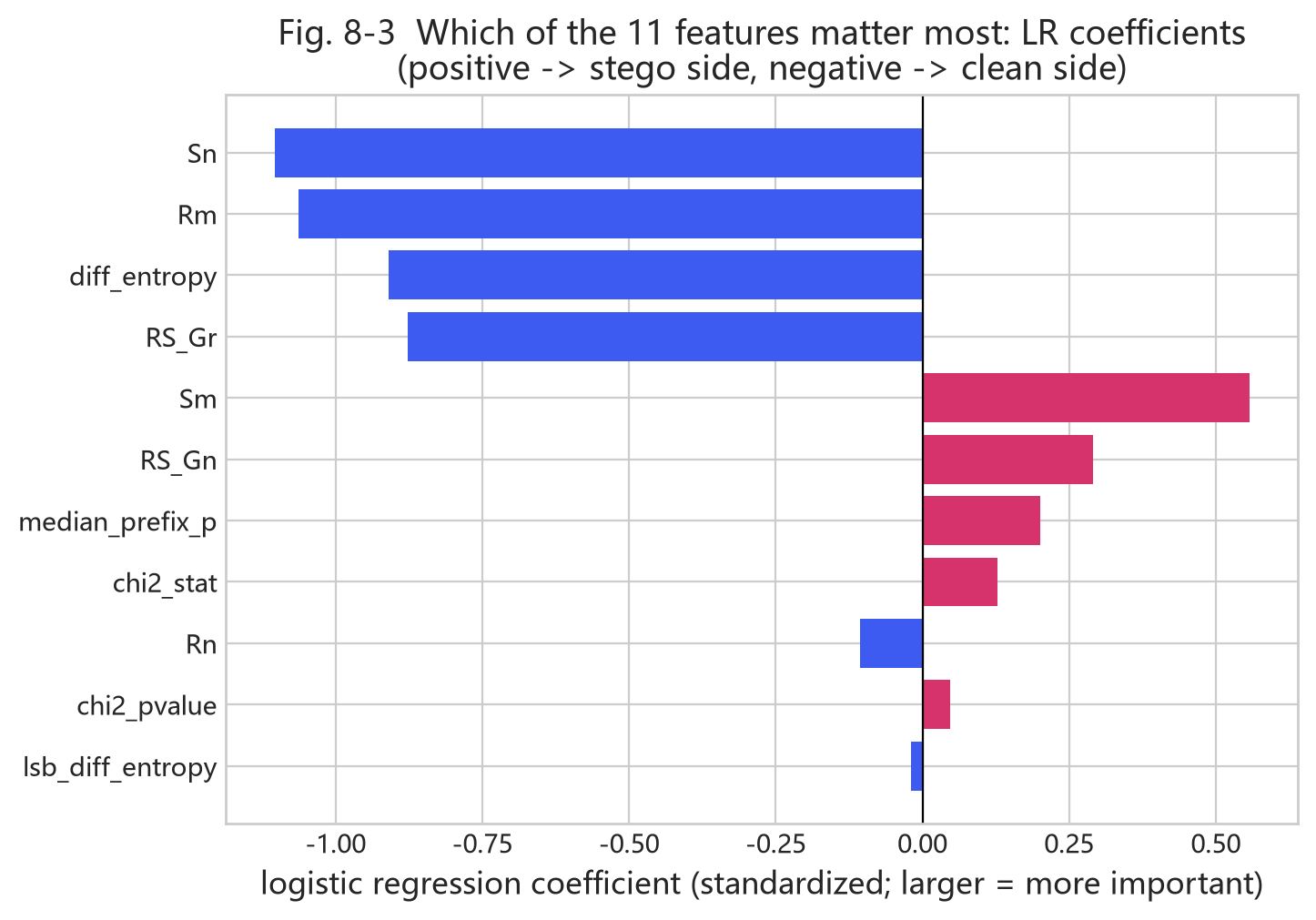
Fig. 8-3 (real data 11-D, standardized LR coefficients: positive (red) pushes toward “hiding”, negative (blue) pulls toward “clean”; larger absolute value = more important. Sn, Rm, diff_entropy, RS_Gr contribute a lot (negative); Sm, RS_Gn, median_prefix_p, chi2_stat contribute a lot (positive))

Reading the figure:

Large absolute coefficients = big influence on the judgement;
Positive coefficients = larger feature value means more hiding; negative the opposite;
This echoes Fig. 8-1: a large Gn means more clean (hence the coefficient direction).

8.4.3 A Crucial Detail: OOF and “Do Not Test Yourself”#

The cross-validation in step 3 is not only to compare models - it also produces a clean, trustworthy score. Its trick: each sample is predicted only by a fold that never saw it, and those predictions are collected (called OOF, out-of-fold). This score is honest - not contaminated by “training and testing on yourself.”

Watch out | The calibration set is for choosing a threshold; the test set is used exactly once. Re-tuning the threshold on the test set dirties it. The project’s train/calibration/test three-layer structure is the rigorous practice industry uses.

8.5 Reading Results: ROC, AUC, and Per-Density Rates#

Beyond the overall AUC (Fig. 7-6), look at per-band (method, p, density) detection rates, because the bands differ a lot.

Fig. 8-5 per-density detection

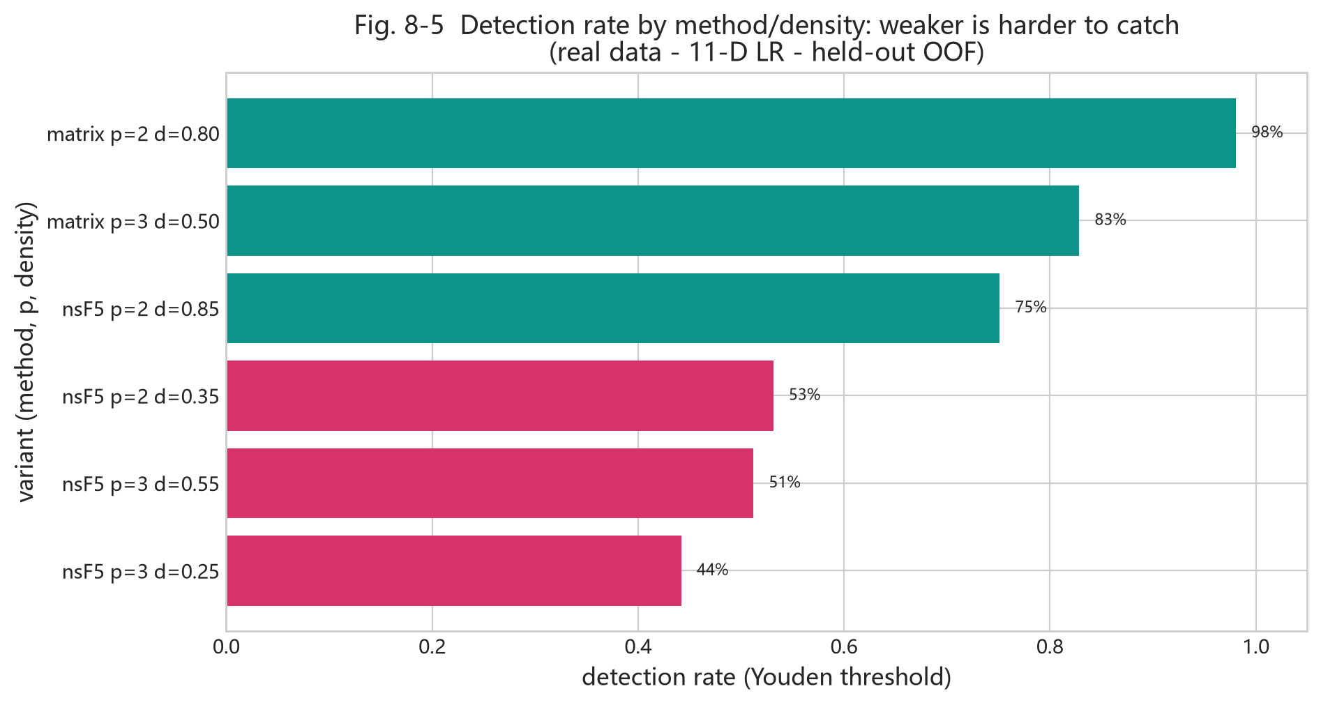
Fig. 8-5 (real data 11-D LR, held-out folds, Youden threshold: detection rate grouped by (method, p, density). Strong densities (matrix p2/p3) near 90%+, weak densities (nsF5 p3 d0.25) clearly lower (around 50%+) - direct evidence that “the weaker the embedding, the harder to detect”)

Back to the code | Compare experiments/data/density_grid.csv (real statistics produced by the chapter-5 experiments): LSB bands are near 100%, matrix p2 d0.80 is about 95%, while weak nsF5 p3 d0.25 reaches only ~47% and nsF5 p3 d0.55 ~55%. This confirms 8.3 - small density means a weak statistical trace, a weak feature signal, so harder to detect - not mysticism.

8.6 Sensitivity: Switching “Strict/Loose” in the GUI#

src/ml_predict.py’s MLPredictor preprocesses the image (grayscale -> 512x512), then auto-selects 11-D or 143-D by the model’s stored feature count, and outputs a hiding probability. “Sensitivity” just means switching the decision threshold:

Sensitivity	ML threshold	Effect
Strict (low FP)	threshold_low_fp	Fewest clean-image errors; more weak hidden missed
Balanced	Youden threshold	Balanced detection vs false positives; default
Loose (high detection)	Youden x 0.75	Catches more weak densities; false positives rise

Against the code - ml_predict.py::_threshold.

if self.sensitivity.startswith("严格"): return float(d.get("threshold_low_fp", d["threshold"]))
if self.sensitivity.startswith("宽松"): return max(0.05, float(d["threshold"]) * 0.75)
return float(d["threshold"])

Tip | “Loose” does not use a new model - it just lowers the decision threshold by 25%. A lower threshold is more aggressive: catches more weakly-hidden images, but raises false positives - the “threshold = strict or loose” from Fig. 7-7/7-8, made concrete.

The GUI’s “Analyze” page shows the heuristic probability and the ML probability side by side and asks you to cross-check, not trust one number - a deliberate honesty feature.

8.7 Experiments: From Training to Single-Image Judgment#

The full pipeline (minutes to tens of minutes, machine dependent)

# 1) generate a dataset (point it at your own photo folder)
python src/make_dataset.py

# 2) train and evaluate
python src/train_model.py

# 3) single-image ML judgment
import sys; sys.path.insert(0, "src")
import numpy as np
from PIL import Image
from ns5_core import embed_string
from ml_predict import get_predictor
a = np.asarray(Image.open("img/cover.png").convert("L"))
s, _, _ = embed_string(a, "ML test", method="nsF5", p=3)
print(get_predictor().predict(s))

Try it | Run an honesty experiment: judge a clean photo (should be near clean), then hide a weak-band message (nsF5 p=3, density near 0.25) and judge again. Watch whether the probability rises only slightly - that is the README warning about weak densities, live.

Against Chapter 7 formulas | Step 3’s predict() is internally: feature $x$ -> weighted sum $z=w·x+b$ -> sigmoid to probability -> compare with threshold for the verdict.

8.8 v1.4.0 Update: SRM, 143-D Features, and Dual Models (2026-09)#

Sections 8.1-8.7 describe the v1.0-v1.3 route: 11-D features with LR/XGB, AUC ~0.75-0.79. v1.4.0 upgraded along three lines: SRM high-pass preprocessing, 143-D v2 features with 12 variants, and finally the dual LightGBM model strategy. The story follows the actual evolution, so the README’s experiment tables make sense.

8.8.1 SRM High-Pass Filtering: v1-Era Same-Source Gain, Cross-Source Loss (not reproduced in the current revision)#

SRM (Spatial Rich Model) is a set of high-pass filter kernels. src/srm_filter.py implements 30 standard kernels, filters the image, takes the maximum absolute response per pixel, clips to +/-4, and rescales into an “enhanced image” that feeds the existing feature extractors. CPU (numpy) and GPU (torch) implementations; switches are make_dataset.py --preprocess srm and the GPU use_srm=True.

Metric	Same-source baseline	Same-source + SRM
5-fold CV-AUC	0.7594	0.7922
Held-out test AUC	0.7811	0.8085
Weak nsF5 p3 d0.25 detection	51.9%	62.5%
nsF5 p2 d0.35 detection	76.0%	90.4%
Low-FP stego detection	41.2%	50.3%
Clean false positives (low-FP thr)	9.6%	9.6%

Watch out (v1-era protocol; not reproduced in the current revision) | In that protocol the gain only appeared within same-source data. In cross-source (campus + full BOSSbase), SRM pulls CPU test AUC from 0.741 down to 0.704 and GPU validation AUC from 0.651 down to 0.572 - high-pass filtering also flattens the differences between cameras/compression sources. So the default model is trained on merged data without SRM, while the SRM campus model is kept separately as campus_srm.

8.8.2 The v2 143-D Feature Set and 12 Variants#

src/featurize_v2.py adds: mean / absolute mean / standard deviation over 30 SRM residuals (90-D), 20 full-image prefix chi-square p-values, 20 LSB-prefix p-values, plus texture_noise and est_rate (2-D): 11 + 90 + 20 + 2 + 20 = 143. Variants grow from 6 to 12: add nsF5 p3 d0.40, matrix p3 d0.40/0.60, and lsb d0.30/0.50/0.70.

Strict A/B (same test-photo groups, 5-fold GroupKFold OOF): the v2 dataset alone adds +0.019; adding 143-D adds another +0.027 (OOF 0.8143, held-out 0.8278), about +0.05 AUC total.

Tip | 143-D is not extra from nowhere - it measures 8.2’s three groups of rulers finer and from more angles: BASE 11 is the backbone; SRM 90 are residual statistics; PREFIX 20 + LSB-PREFIX 20 are the chi-square test “split into 20 segments + LSB version”. Still measuring the same thing - the statistical trace.

8.8.3 Real JPEG Clean Images Expose a Deployment Problem - and the Fix#

The v2 logistic model scored well inside its training distribution, but on real JPEG clean photos it flagged almost everything as 1.0: SRM residuals react strongly to JPEG high-frequency noise. The fix: add 414 real JPEG clean photos to the training corpus, producing dataset_campus_v2_jpeg.csv, then grid-tune LightGBM. Corrected 2026-09-14: those rows were originally given independent photo_ids while their features were bit-identical to the matching clean row (a duplicate), so a source photo could straddle the train/validation split; the corpus was also built with GPU features that scaled pixels by 1/255 before the high-pass filters, differing from the CPU inference path by ~30x. Both are fixed and rerun (see experiments/add_jpeg_clean.py and docs/RESULTS.md). Current numbers: 143-D held-out 0.8939, 8-split 0.8980, weak nsF5 p3 d0.25 50.0%; 53-D 0.8391 / 0.8461 / 41.4%.

Tip | This is a live distribution shift case: the model learns well on “campus PGM/BMP grayscale” then breaks on “real JPEG camera noise.” The project fixes it by adding real JPEG clean images to training - training data must cover the real deployment scenario, or the score is self-congratulation.

8.8.4 Dual-version Deployment: 143d Robust vs 53d Interpretable#

Interpretability, recomputed after the audit: within the 143-D set the 90 SRM dimensions carry 52.6% of the LightGBM gain (BASE 11: 20.7%, LSB PREFIX 20: 20.6%, PREFIX 20: 6.2%); ablation shows that dropping them costs 0.05 AUC (5-fold OOF 0.9010 -> 0.8513). So two models are kept:

Dimension	143d default (robust)	53d interpretable
Features	BASE11 + SRM90 + PREFIX20 + LSB-PREFIX20 + TEX/EST2	Same minus SRM90 (53-D)
8-split mean AUC	0.8980	0.8461
Held-out AUC	0.8939	0.8391
Weak nsF5 p3 d0.25	50.0%	41.4%
Real-JPEG clean OOD	9.58% (n=1514, 95% CI 8.20-11.16%)	28.86% (26.64-31.20%)
Best for	Deployment / mixed domains / real images	Teaching / defenses / per-image explanations (AUC ~0.05 lower)

MLPredictor() loads 143d by default; pass model_path to switch to 53d. Inference auto-selects 11-D or 143-D from the model metadata. GUI model switching is still planned; for now, switch via the API:

Switching between the dual models

from ml_predict import MLPredictor
 
# default: 143d robust model (models/stego_classifier.joblib)
pred_143 = MLPredictor()
 
# 53d interpretable model (SRM 90 removed; slightly lower AUC, fully interpretable)
pred_53 = MLPredictor(
    model_path='models/stego_classifier_v2_jpeg_lgb_51d.joblib',
    clip_outliers=False)
 
r = pred_53.predict(img)
# {'probability': ..., 'verdict': ..., 'threshold': ...}

Try it | Experiment: train on dataset_campus_v2_jpeg.csv (set $env:DS_FILES), then compare 143d vs 53d on real JPEG clean photos and on weak nsF5 p3 d0.25 images. Put the AUC and OOD behavior into your report.

Watch out | The v2/53d models are only reliable near their training distribution. For a brand-new camera or compression source, run a small OOD test before deployment.

8.9 Summary and Self-Check#

One sentence: under “small samples + weak signals”, domain features + simple classifiers are more reliable than a raw CNN; and the features set the ceiling - the classifier merely mines the signal in them.

The 11 features = RS family (Gn collapse) + chi-square family (gray pairs flattened) + entropy/randomness baseline (spotting naturally messy images); see Fig. 8-1/8-2.
The four classifiers (LR/RF/GB/XGB) differ little on the 11-D features (Fig. 8-4); what really separates is features (Fig. 8-3) and data.
Train/calibration/test three-layer structure + GroupKFold is the skeleton of experimental trust;
The weaker, the harder to detect (Fig. 8-5); detection has a physical ceiling;
Cross-check ML probability with heuristics; since v1.4 dual models are strong, but real-JPEG OOD validation remains mandatory (8.8).

Think about it | One photo has 7 samples. Why is a random 80/20 split not acceptable? Design a minimal example showing how much leakage can inflate AUC. One layer deeper: if you lower the “Loose” threshold again in 8.6, how does the false-positive rate change? Why are “catch more” and “false-positive less” always in tension? Finally: if you had 100,000 independent photos, would you still stick with “features instead of a raw CNN”? Why?